FiveThirtyEight’s Riddler Express#
From Taylor Firman comes an opportunity to make baseball history:
This year, Major League Baseball announced it will play a shortened 60-game season, as opposed to the typical 162-game season. Baseball is a sport of numbers and statistics, and so Taylor wondered about the impact of the season’s length on some famous baseball records.
Some statistics are more achievable than others in a shortened season. Suppose your true batting average is .350, meaning you have a 35 percent chance of getting a hit with every at-bat. If you have four at-bats per game, what are your chances of batting at least .400 over the course of the 60-game season?2 And how does this compare to your chances of batting at least .400 over the course of a 162-game season?
Plan#
This riddle should be pretty straight forward to solve statistically and with simulations, so I will do both.
Setup#
knitr::opts_chunk$set(echo = TRUE, comment = "#>", cache = FALSE, dpi = 400)

library(mustashe)
library(tidyverse)
library(conflicted)

# Handle any namespace conflicts.
conflict_prefer("filter", "dplyr")
conflict_prefer("select", "dplyr")

# Default 'ggplot2' theme.
theme_set(theme_minimal())

# For reproducibility.
set.seed(123)
Statistical solution#
This is a simple binomial system: at each at bat, the player either gets a hit or not. If their real batting average is 0.350, that means the probability of them getting a hit during each at bat is 35%. Thus, according the the Central Limit Theorem, given a sufficiently large number of at bats, the frequency of a hit should be 35%. This is because the distribution converges towards the mean. However, at smaller sample-sizes, the distribution is more broad, meaning that the observed batting average has a greater chance of being further away from the true value.
First, let’s answer the riddle. The solution is just the probability of
observing a batting average of 0.400 or greater. The first value is
computed using dbinom() and the second cumulative probability is
calculated using pbinom(), setting lower.tail = FALSE to get the
tail above 0.400.
num_at_bats <- 60 * 4
real_batting_average <- 0.350
target_batting_average <- 0.400

prob_at_400 <- dbinom(x = target_batting_average * num_at_bats,
                      size = num_at_bats,
                      prob = real_batting_average)
prob_above_400 <- pbinom(q = target_batting_average * num_at_bats,
                         size = num_at_bats,
                         prob = real_batting_average,
                         lower.tail = FALSE)
prob_at_400 + prob_above_400
#> [1] 0.06083863
Under the described assumptions, there is a 6.1% chance of reaching a batting average of 0.400 in the shorter season.
For comparison, the chance for a normal 162-game season is calculated below. Because $0.400 \times 162 \times 4$ is a non-integer value, an exact 0.400 batting average cannot be obtained. Therefore, only the probability of a batting average greater than 0.400 needs to be calculated.
num_at_bats <- 162 * 4
real_batting_average <- 0.350
target_batting_average <- 0.400

prob_above_400 <- pbinom(q = target_batting_average * num_at_bats,
                         size = num_at_bats,
                         prob = real_batting_average,
                         lower.tail = FALSE)
prob_above_400
#> [1] 0.003789922
Over 162 games, there is a 0.4% chance of achieving a batting average of at least 0.400.
Simulation#
The solution to this riddle could also be found by simulating a whole bunch of seasons with the real batting average of 0.350 and then just counting how frequently the simulations resulted in an observed batting average of 0.400.
A single season can be simulated using the rbinom() function where n
is the number of seasons to simulate, size takes the number of at
bats, and prob takes the true batting average. The returned value is a
sampled number of hits (“successes”) over the season from the binomial
distribution.
The first example shows the observed batting average from a single season.
num_at_bats <- 60 * 4
real_batting_average <- 0.350
target_batting_average <- 0.400

rbinom(n = 1, size = num_at_bats, prob = real_batting_average) / num_at_bats
#> [1] 0.3375
The n = 1 can just be replaced with a large number to simulate a bunch
of seasons. The average batting average over these seasons should be
close to the true batting average.
n_seasons <- 1e6  # 1 million simulations.
sim_res <- rbinom(n = n_seasons,
                  size = num_at_bats,
                  prob = real_batting_average)

sim_res <- sim_res / num_at_bats

# The average batting average is near the true batting average of 0.350.
mean(sim_res)
#> [1] 0.3500121
The full distribution of batting averages over the 1 million simulations is shown below.
tibble(sims = sim_res) %>%
    ggplot(aes(x = sims)) +
    geom_density(color = "black", fill = "black", adjust = 2,
                 alpha = 0.2, size = 1.2, ) +
    geom_vline(xintercept = target_batting_average,
               color = "tomato", lty = 2, size = 1.2) +
    scale_y_continuous(expand = expansion(mult = c(0.01, 0.02))) +
    theme(plot.title = element_text(hjust = 0.5)) +
    labs(x = "1 million simulated season batting averages",
         y = "probability density",
         title = "Distribution of simulated batting averages in a 60-game season")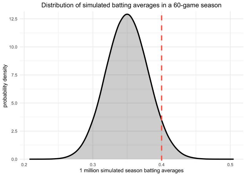
The answer from the simulation is pretty close to the actual answer.
mean(sim_res >= 0.40)#> [1] 0.060813
One last visualization I want to do demonstrates why the length of the
season matters to the distribution. Instead of using rbinom() to
simulate the number of successes over the entire season, I use it below
to simulate a season’s-worth of individual at bats, returning a vector
of 0’s and 1’s. I then plotted the cumulative number of hits at each at
bat and colored the line by the running batting average.
The coloring shows how the batting average was more volatile when there were fewer at bats.
sampled_at_bats <- rbinom(60*4, 1, 0.35)
tibble(at_bat = sampled_at_bats) %>%
    mutate(i = row_number(),
           cum_total = cumsum(at_bat),
           running_avg = cum_total / i) %>%
    ggplot(aes(x = i, y = cum_total)) +
    geom_line(aes(color = running_avg), size = 1.2) +
    scale_color_viridis_c() +
    theme(plot.title = element_text(hjust = 0.5),
          legend.position = c(0.85, 0.35)) +
    labs(x = "at bat number",
         y = "total number of hits",
         color = "batting average",
         title = "Running batting average over a simulated season")
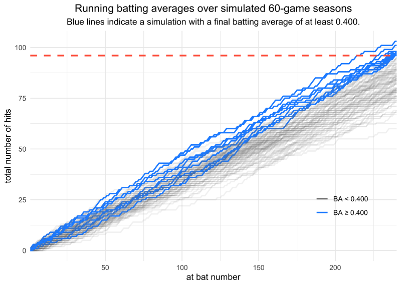
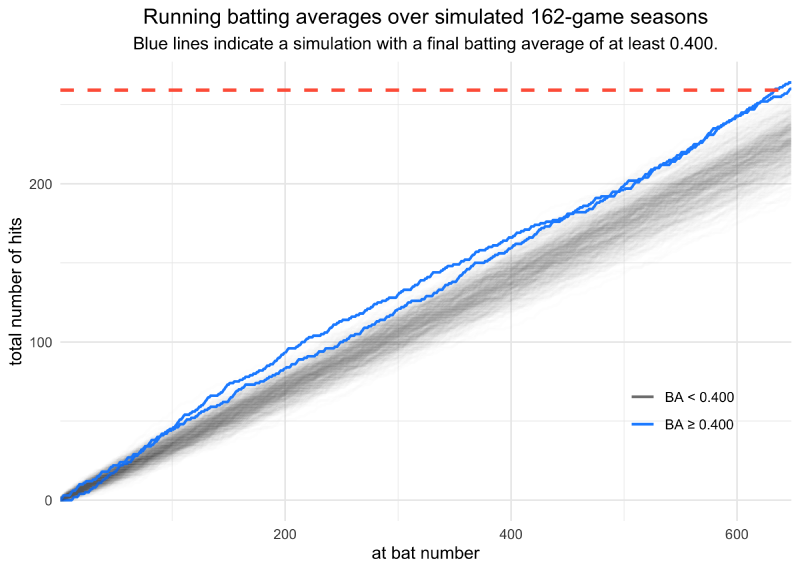
The following two plots do the same analysis many times to simulate many seasons and color the lines by whether or not the final batting average was at or above 0.400. As there are more games, the running batting averages, which are essentially biased random walks, regress towards the true batting average. (Note that I had to do 500 simulations for the 162-game season to get any simulations with a final batting average above 0.400.)
simulate_season_at_bats <- function(num_at_bats) {
    sampled_at_bats <- rbinom(num_at_bats, size = 1, prob = 0.35)
    tibble(result = sampled_at_bats) %>%
        mutate(at_bat = row_number(),
               cum_total = cumsum(result),
               running_avg = cum_total / at_bat)
}

tibble(season = 1:100) %>%
    mutate(season_results = map(season, ~ simulate_season_at_bats(60 * 4))) %>%
    unnest(season_results) %>%
    group_by(season) %>%
    mutate(
        above_400 = 0.4 <= running_avg[which.max(at_bat)],
        above_400 = ifelse(above_400, "BA ≥ 0.400", "BA < 0.400")
    ) %>%
    ungroup() %>%
    ggplot(aes(x = at_bat, y = cum_total)) +
    geom_line(aes(group = season, color = above_400,
                  alpha = above_400),
              size = 0.8) +
    geom_hline(yintercept = 0.4 * 60 * 4,
               color = "tomato", lty = 2, size = 1) +
    scale_color_manual(values = c("grey50", "dodgerblue")) +
    scale_alpha_manual(values = c(0.1, 1.0), guide = FALSE) +
    scale_x_continuous(expand = c(0, 0)) +
    theme(plot.title = element_text(hjust = 0.5),
          plot.subtitle = element_text(hjust = 0.5),
          legend.position = c(0.85, 0.25)) +
    labs(x = "at bat number",
         y = "total number of hits",
         color = NULL,
         title = "Running batting averages over simulated 60-game seasons",
         subtitle = "Blue lines indicate a simulation with a final batting average of at least 0.400.")