FiveThirtyEight’s Riddler Express#
The following article has been updated to fix an error identified by several readers. Thank you for your help!
In Riddler City, the city streets follow a grid layout, running north-south and east-west. You’re driving north when you decide to play a little game. Every time you reach an intersection, you randomly turn left or right, each with a 50 percent chance.
After driving through 10 intersections, what is the probability that you are still driving north?
Extra credit: Now suppose that at every intersection, there’s a one-third chance you turn left, a one-third chance you turn right and a one-third chance you drive straight. After driving through 10 intersections, now what’s the probability that you are still driving north?
Plan#
This puzzle could be solved analytically, but that would require a lot more thought than just simulating it. I will try to make the algorithm generalizable to also be able to solve the extra credit problem without too many changes.
Setup#
knitr::opts_chunk$set(echo = TRUE, comment = "#>", cache = TRUE, dpi = 400)

library(tidyverse)
library(conflicted)

# Handle any namespace conflicts.
conflict_prefer("filter", "dplyr")
conflict_prefer("select", "dplyr")

# Default 'ggplot2' theme.
theme_set(theme_minimal())

# For reproducibility.
set.seed(0)
A single simulation#
The abstraction#
The code for the simulation itself is very simple and mainly contained
within two functions, simulate_one_drive() that coordinates everything
and adjust_direction() that turns the player based on the current
direction and random turn. More on these in a second.
The tricky part for this simulation was choosing an abstraction. My first few attempts relied on keeping track of the cardinal direction (i.e. north, south, east, and west), randomly deciding the turn, and then updating the cardinal direction based on the turn. But this was annoyingly complicated because the effect of left or right on the cardinal direction depends on the direction, itself. Therefore, it looked like I would need to write a massive (read “error-prone”) if-else statement.
After quite a bit of thought and diagramming, I realized I could use angles to solve the problem. If I set north as $\frac{\pi}{2}$, then a left turn would be equivalent to adding $\frac{\pi}{2}$ and turning right would be equivalent to subtracting $\frac{\pi}{2}$. And this would be true regardless of the current direction!

Using this approach, I decided to just keep track of the angle of the current direction and ignore actually traveling through the city. I could just calculate this afterwards, if needed.
The main process#
Finally, we can get to the code. The simulate_one_drive() function
takes probabilities for turning left (l), right (r), or continuing
straight (s) and an argument for the number of steps in the simulation
(n_steps).
Right away, the starting direction is defined as $\frac{1}{2}$. I left out $\pi$ from the simulation because I never actually need radians, just a relative unit for the angle. Therefore, instead of ranging from 0 to $2\pi$, the “angle” ranges from 0 to 2. Multiplying by $\pi$ later can return the radians.
Before the for-loop, there is a quick check to make sure the probabilities sum to 1.
Finally, the tracker is instantiated as a data frame with the interaction, current direction, and the choice of turn (“S” for straight to begin with).
In each step of the for-loop
- a turn is randomly chosen according to their predetermined likelihoods,
- the direction is changed according to the result of the random
selection using the
adjust_direction()function (more in a second), - the tracker is updated with the current step.
The tracker is returned as the result of the simulation.
# Simulate one drive.
simulate_one_drive <- function(l, r, s, n_steps = 10) {
    # Start facing "North".
    dir <- 1/2

    # Check that the total probability of turning choices is 1.
    stopifnot(sum(c(l, r, s)) == 1)

    # Start the tracker.
    tracker <- update_tracker(tibble(), 0, dir, "S")

    # Take `n_steps` for the simulation.
    for (i in seq(1, n_steps)) {
        next_turn <- sample(c("L", "R", "S"), 1, prob = c(l, r, s))
        dir <- adjust_direction(dir, next_turn)
        tracker <- update_tracker(tracker, i, dir, next_turn)
    }

    return(tracker)
}
The update tracker function is just a convenience function for adding rows to a data frame of the current state of the simulation at each step.
# Update the tracker data frame.
update_tracker <- function(tracker, i, dir, turn) {
    bind_rows(
        tracker,
        tibble(i = i, direction = dir, turn = turn)
    )
}
The adjust_direction() function takes a current direction (curr_dir)
and which way to turn (turn). It then adds $\frac{1}{2}$ to turn
left ("L") or subtracts $\frac{1}{2}$ to turn right ("R"). The
original direction is returned to continue straight ("S").
Note that the reason this function is so simple is not because I did anything clever with the code, but instead it’s because the abstraction is so natural to the problem.
# Adjust the current direction `curr_dir` based off of the `turn`.
adjust_direction <- function(curr_dir, turn) {
    new_dir <- curr_dir
    if (turn == "L") {
        new_dir <- curr_dir + 0.5
    } else if (turn == "R") {
        new_dir <- curr_dir - 0.5
    } else if (turn == "S") {
        new_dir <- curr_dir
    } else {
        stop(paste0("The change in direction '", turn, "' is not recognized."))
    }
    return(new_dir)
}
An example simulation#
Below I run a single example simulation and receive back the tracker.
set.seed(0)
example_sim <- simulate_one_drive(0.5, 0.5, 0, n_steps = 10)
example_sim
#> # A tibble: 11 x 3
#>        i direction turn
#>    <dbl>     <dbl> <chr>
#>  1     0       0.5 S
#>  2     1       1   L
#>  3     2       0.5 R
#>  4     3       0   R
#>  5     4       0.5 L
#>  6     5       1   L
#>  7     6       0.5 R
#>  8     7       1   L
#>  9     8       1.5 L
#> 10     9       2   L
#> 11    10       2.5 L
From the direction column, we can calculate the change in $x$ and
$y$ by converting from polar coordinates $(r, \theta)$ to cartesian
coordinates $(x,y)$:
$x = r \times \cos(\theta)$
$y = r \times \sin(\theta)$
example_sim2 <- example_sim %>%
    mutate(dx = round(1 * cos(direction * pi)),
           dy = round(1 * sin(direction * pi)))
example_sim2
#> # A tibble: 11 x 5
#>        i direction turn     dx    dy
#>    <dbl>     <dbl> <chr> <dbl> <dbl>
#>  1     0       0.5 S         0     1
#>  2     1       1   L        -1     0
#>  3     2       0.5 R         0     1
#>  4     3       0   R         1     0
#>  5     4       0.5 L         0     1
#>  6     5       1   L        -1     0
#>  7     6       0.5 R         0     1
#>  8     7       1   L        -1     0
#>  9     8       1.5 L         0    -1
#> 10     9       2   L         1     0
#> 11    10       2.5 L         0     1
With the change in $x$ and $y$ after each turn in the simulation,
the actual position of the car on the grid can be calculated. This is
accomplished by using the
accumulate2()
function from the ‘purrr’
package.
calculate_position <- function(pos, dx, dy) {
    new_pos <- pos
    new_pos$x <- pos$x + dx
    new_pos$y <- pos$y + dy
    return(new_pos)
}

example_sim3 <- example_sim2 %>%
    mutate(pos = accumulate2(dx, dy,
                             calculate_position,
                             .init = list(x = 0, y = 0))[-1],
           x = map_dbl(pos, ~ .x$x),
           y = map_dbl(pos, ~ .x$y))
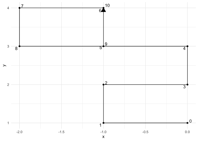
Finally, to have a more satisfying visualization of the simulation, we can plot the $x$ and $y$ positions for each turn.
example_sim3 %>%
    ggplot(aes(x, y)) +
    geom_path(group = "a",
              arrow = arrow(length = unit(4, "mm"), ends = "last", type = "closed")) +
    geom_point() +
    ggrepel::geom_text_repel(aes(label = i))
To facilitate further analysis of the results of simulations, I packaged
the above steps into a single function
simulation_results_to_cartesian_positions().
calculate_position <- function(pos, dx, dy) {
    new_pos <- pos
    new_pos$x <- pos$x + dx
    new_pos$y <- pos$y + dy
    return(new_pos)
}

simulation_results_to_cartesian_positions <- function(df) {
    df %>%
        mutate(dx = round(1 * cos(direction * pi)),
               dy = round(1 * sin(direction * pi)),
               pos = accumulate2(dx, dy,
                                 calculate_position,
                                 .init = list(x = 0, y = 0))[-1],
               x = map_dbl(pos, ~ .x$x),
               y = map_dbl(pos, ~ .x$y))
}

simulation_results_to_cartesian_positions(example_sim)
#> # A tibble: 11 x 8
#>        i direction turn     dx    dy pos                  x     y
#>    <dbl>     <dbl> <chr> <dbl> <dbl> <list>           <dbl> <dbl>
#>  1     0       0.5 S         0     1 <named list [2]>     0     1
#>  2     1       1   L        -1     0 <named list [2]>    -1     1
#>  3     2       0.5 R         0     1 <named list [2]>    -1     2
#>  4     3       0   R         1     0 <named list [2]>     0     2
#>  5     4       0.5 L         0     1 <named list [2]>     0     3
#>  6     5       1   L        -1     0 <named list [2]>    -1     3
#>  7     6       0.5 R         0     1 <named list [2]>    -1     4
#>  8     7       1   L        -1     0 <named list [2]>    -2     4
#>  9     8       1.5 L         0    -1 <named list [2]>    -2     3
#> 10     9       2   L         1     0 <named list [2]>    -1     3
#> 11    10       2.5 L         0     1 <named list [2]>    -1     4
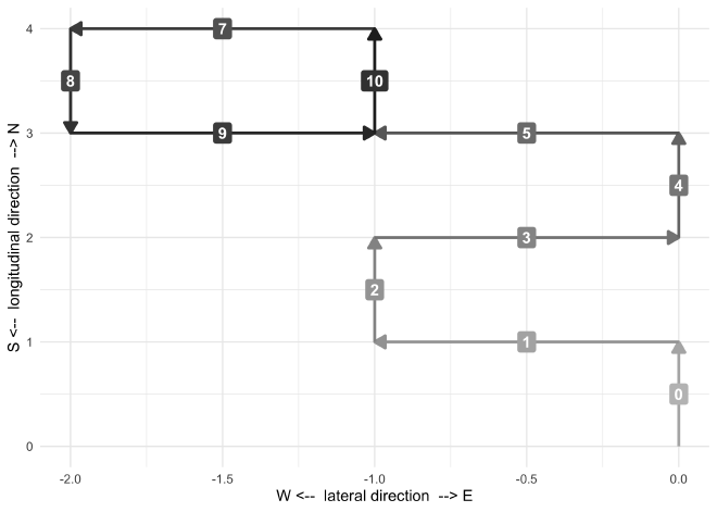
I also made a more expressive plotting function plot_simulation() that
shows the direction at each step.
plot_simulation <- function(df) {
    df %>%
        group_by(sim) %>%
        mutate(x_start = dplyr::lag(x, default = 0),
               y_start = dplyr::lag(y, default = 0)) %>%
        ungroup() %>%
        ggplot() +
        geom_segment(aes(x = x_start, y = y_start, xend = x, yend = y,
                         color = i, group = sim),
                     arrow = arrow(length = unit(3, "mm"), type = "closed"),
                     alpha = 1.0, size = 1) +
        geom_label(aes((x_start + x) / 2, (y_start + y) / 2, label = i, fill = i),
                   color = "white", label.size = 0, fontface = "bold") +
        scale_color_gradient(low = "grey70", high = "grey15", guide = FALSE) +
        scale_fill_gradient(low = "grey75", high = "grey25", guide = FALSE) +
        labs(x = "W <--  lateral direction  --> E",
             y = "S <--  longitudinal direction  --> N")
}

example_sim %>%
    simulation_results_to_cartesian_positions() %>%
    mutate(sim = 1) %>%
    plot_simulation()
The simulation#
Finally, we can run a bunch of simulations and answeer the original question:
After driving through 10 intersections, what is the probability that you are still driving north?
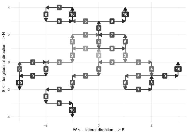
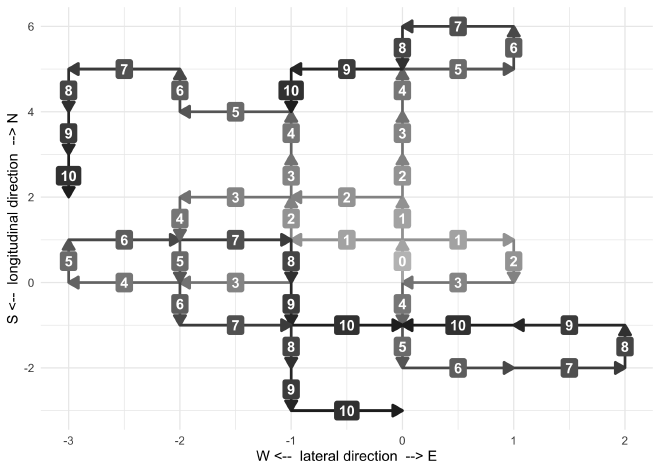
First, lets plot the results of 5 simulations to ensure that the simulation is working as expected over multiple runs.
set.seed(0)
tibble(sim = 1:5) %>%
    mutate(res = map(sim, ~ simulate_one_drive(0.5, 0.5, 0, n_steps = 10)),
           res = map(res, simulation_results_to_cartesian_positions)) %>%
    unnest(res) %>%
    plot_simulation()
With that check done, we are ready to run a few thousand simulations.
set.seed(0)
N_sims <- 1e4

simulation_results <- tibble(sim = 1:N_sims) %>%
    mutate(res = map(sim, ~ simulate_one_drive(0.5, 0.5, 0, n_steps = 10)))

simulation_results
#> # A tibble: 10,000 x 2
#>      sim res
#>    <int> <list>
#>  1     1 <tibble [11 × 3]>
#>  2     2 <tibble [11 × 3]>
#>  3     3 <tibble [11 × 3]>
#>  4     4 <tibble [11 × 3]>
#>  5     5 <tibble [11 × 3]>
#>  6     6 <tibble [11 × 3]>
#>  7     7 <tibble [11 × 3]>
#>  8     8 <tibble [11 × 3]>
#>  9     9 <tibble [11 × 3]>
#> 10    10 <tibble [11 × 3]>
#> # … with 9,990 more rows
Now we have a long data frame with nested data frames, each one
respresenting the results of a single simulation. We now want to tell if
the final direction was pointing north. However, there is one subtle
problem: $\frac{\pi}{2} = \frac{5\pi}{2} = \frac{9\pi}{2} = …$.
There are many (infinite) possible angles that all point north.
Therefore, I wrote the reduce_angle() function to reduce any angle to
lie within 0 and 2 (because we removed the constant $\pi$ from the
angle of direction).
# Reduce the angle from an value to between 0 and 2.
reduce_angle <- function(theta) {
    theta - (2 * trunc(theta / 2))
}
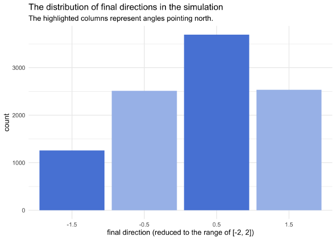
Now, we can unnest the simulation results, take the last direction, and see if it is pointing north.
simulation_results <- simulation_results %>%
    unnest(res) %>%
    filter(i == 10) %>%
    mutate(reduced_direction = reduce_angle(direction))

prob_north <- sum(simulation_results$reduced_direction %in% c(0.5, -1.5)) / N_sims
The probability of still facing north after randomly turning left and right at each intersection is 0.495.
is_north_pal <- c("TRUE" = "#5887db", "FALSE" = "#a7bfeb")

simulation_results %>%
    count(reduced_direction) %>%
    mutate(is_north = reduced_direction %in% c(0.5, -1.5)) %>%
    ggplot(aes(x = factor(reduced_direction), y = n)) +
    geom_col(aes(fill = is_north)) +
    scale_fill_manual(values = is_north_pal, guide = FALSE) +
    labs(x = "final direction (reduced to the range of [-2, 2])",
         y = "count",
         title = "The distribution of final directions in the simulation",
         subtitle = "The highlighted columns represent angles pointing north.")
Extra credit#
Since I allowed for a probability of going straight in the
simulate_one_drive() function, solving the extra credit problem
requires no change to the code other than a single argument value.
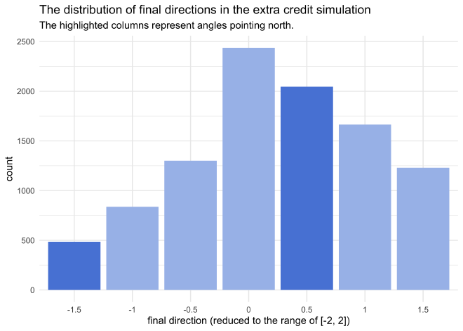
Extra credit: Now suppose that at every intersection, there’s a one-third chance you turn left, a one-third chance you turn right and a one-third chance you drive straight. After driving through 10 intersections, now what’s the probability that you are still driving north?
set.seed(0)
tibble(sim = 1:5) %>%
    mutate(res = map(sim, ~ simulate_one_drive(1/3, 1/3, 1/3, n_steps = 10)),
           res = map(res, simulation_results_to_cartesian_positions)) %>%
    unnest(res) %>%
    plot_simulation()
set.seed(0)

simulation_results_ec <- tibble(sim = 1:N_sims) %>%
    mutate(res = map(sim, ~ simulate_one_drive(1/3, 1/3, 1/3, n_steps = 10))) %>%
    unnest(res) %>%
    filter(i == 10) %>%
    mutate(reduced_direction = reduce_angle(direction))

prob_north <- sum(simulation_results_ec$reduced_direction %in% c(0.5, -1.5)) / N_sims
The probability of still facing north after randomly turning left, right, or continuing straight at each intersection is 0.253.
simulation_results_ec %>%
    count(reduced_direction) %>%
    mutate(is_north = reduced_direction %in% c(0.5, -1.5)) %>%
    ggplot(aes(x = factor(reduced_direction), y = n)) +
    geom_col(aes(fill = is_north)) +
    scale_fill_manual(values = is_north_pal, guide = FALSE) +
    labs(x = "final direction (reduced to the range of [-2, 2])",
         y = "count",
         title = "The distribution of final directions in the extra credit simulation",
         subtitle = "The highlighted columns represent angles pointing north.")
