Here, I demonstrate how to find the point where two histograms overlap. While this is an approximation, it seems to have a very high level of precision.
Prepare simulated data#
I created two data sets, gamma_dist and norm_dist, which are made up of a different number of values sampled randomly from a gamma distribution and normal distribution, respectively. I specicially made the data sets different sizes to make the point that this method is still applicable.
library(tibble)
set.seed(0)
gamma_dist <- rgamma(1e5, shape = 2, scale = 2)
norm_dist <- rnorm(5e5, mean = 20, sd = 5)
df <- tibble(
x = c(gamma_dist, norm_dist),
original_dataset = c(rep("gamma_dist", 1e5), rep("norm_dist", 5e5))
)
df
#> # A tibble: 600,000 x 2
#> x original_dataset
#> <dbl> <chr>
#> 1 6.89 gamma_dist
#> 2 2.25 gamma_dist
#> 3 1.30 gamma_dist
#> 4 4.10 gamma_dist
#> 5 7.77 gamma_dist
#> 6 5.08 gamma_dist
#> 7 4.58 gamma_dist
#> 8 2.30 gamma_dist
#> 9 1.36 gamma_dist
#> 10 1.67 gamma_dist
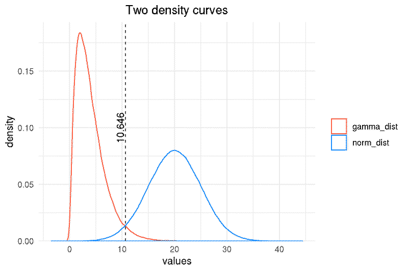
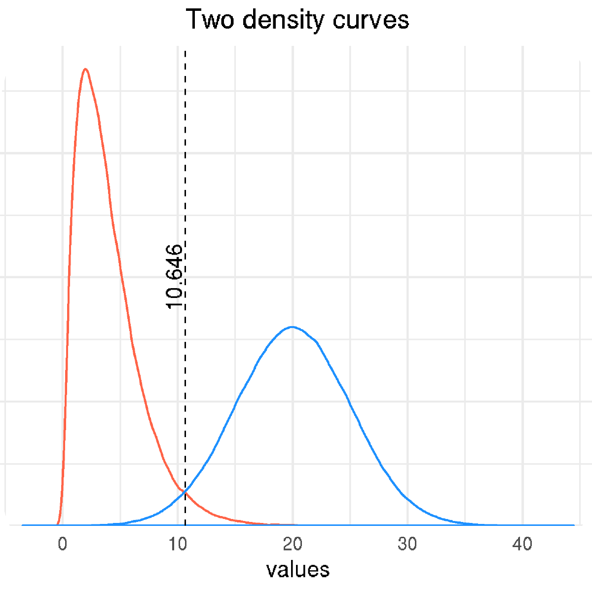
#> # … with 599,990 more rowsI used ‘ggplot2’ to plot the densities of the two data sets. The gamma distribution is in red and the normal distribution is in blue. I broke the creation of the plot into two steps: the essential step to create the density curves, and the styling step to make the plot look nice. Of course, these could be combined into a single long ggplot statement.
library(ggplot2)

p <- ggplot(df) +
  geom_density(aes(x = x, color = original_dataset))

p <- p +
  scale_y_continuous(expand = expand_scale(mult = c(0, 0.05))) +
  scale_color_manual(values = c("tomato", "dodgerblue")) +
  theme_minimal() +
  theme(
      legend.title = element_blank(),
      plot.title = element_text(hjust = 0.5)
  ) +
  labs(x = "values",
       title = "Two density curves")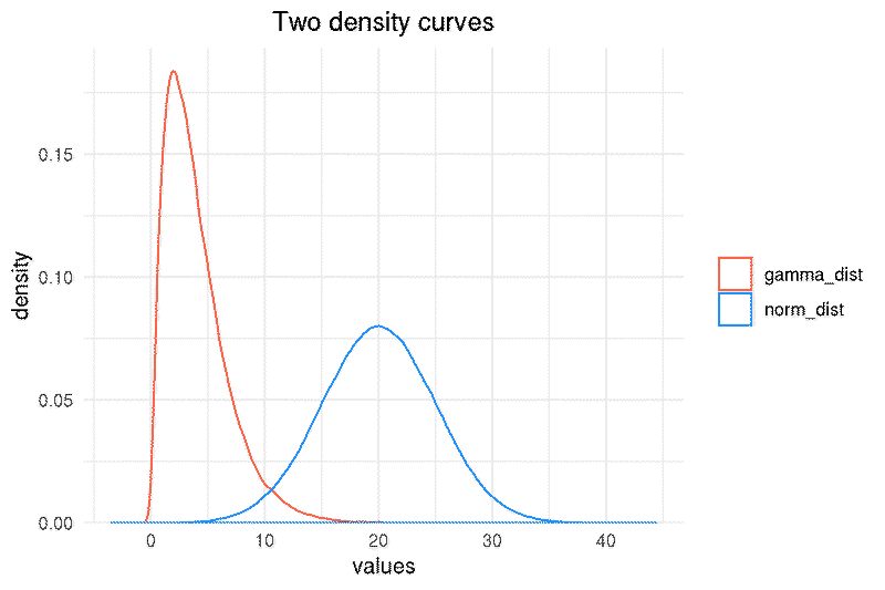
Finding the point of intersection#
To find the point of intersection, I first binned the data sets using density. It is essential to use the same from and to values for each data set. The density function creates 512 bins, thus, providing the same starting and ending parameters makes density use the same bins for each data set.
from <- 0
to <- 40
gamma_density <- density(gamma_dist, from = from, to = to)
norm_density <- density(norm_dist, from = from, to = to)
The final step was to find where the density of the gamma distribution was less than the normal distribution. Therefore, I applied this logic to create the boolean vector idx. I also included two other filters to contain the result between 5 to 20 because, from the plot above, I can see that the intersection falls within this range.
idx <- (gamma_density$y < norm_density$y) &
       (gamma_density$x > 5) &
       (gamma_density$x < 20)
poi <- min(gamma_density$x[idx])
poi
#> 10.64579
That’s it, the point of intersection has been approximated to a high precision. A vertical line was added to the plot below at poi.
p <- p +
  geom_vline(xintercept = poi, linetype = 2, size = 0.3, color = "black") +
  annotate(geom = "text", label = round(poi, 3),
           x = poi - 1, y = 0.1, size = 4, angle = 90)